Separating the Sources of Randomness in Neural Networks at Initialization Time

Preactivation distributions computed over weight randomness (red histograms) and sample randomness (solid histograms) in random ReLU networks initialized with Kaiming initialization
Initialize your network to preserve the variance of neurons across layers.
This prescription is wide spread in the deep learning community and its easy to see why. Not only is it effective, but it is simple to implement, and simple to understand.
For nets with ReLU nonlinearity, we implement this prescription by drawing weights from a zero mean distribution with variance $\frac{2}{\text{fan_in}}$. This is known as Kaiming initialization. Normalization schemes like Batch/Layer/Group/etc. Norm make variance preservation even easier to implement; by design they normalize neurons so they are zero mean and unit variance at init time.
But there is a subtlely here, over what distribution are the mean and variance computed? Kaiming preserves the variance when computed over randomness in weights. Batch Norm normalizes neurons using minibatch statistics. Layer Norm uses the mean and variance over a layer. Group Norm uses mean and variance computed over a group (basically a subset of neurons in a layer).
In this post, we’ll identify two fundamental sources of randomness at initialization time: network randomness (randomness in weight configurations), and sample randomness (randomness in the input distribution). We’ll show that neuron distributions arising from the two sources can be very different from each other.
As expected, we find that every neuron is zero mean and has the same variance over random network configurations. However, if you generate a single network, and compute the mean and variance of a neuron over the sample distribution only, we find the variance decays with depth! With two mean-field approximations, we can actually compute the rate at which this variance decays.
This post is mostly derived from a paper my advisor and I wrote. Some of the calculations are different in an attempt to be less formal but hopefully simpler to understand.
TL;DR: Neurons can have very different distributions when they are computed over weight randomness compared to when they are computed over sample randomness. In a random Kaiming-initialized ReLU network, the neuron variance computed over weight randomness is the same in every layer but the variance of neurons computed over samples can decay to zero with depth!
Setup
We are going to examine preactivation distributions in the simplest (most boring) network we can. Our network will be a 50 layer, fully connected, 1024 neuron wide, feedforward network:
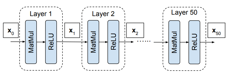
The forward pass of our network is defined by:
\[\mathbf{y}_l = \mathbf{W}_l \mathbf{x}_{l-1} \qquad \mathbf{x}_l = f(\mathbf{y}_l)\]where $\mathbf{y}_l$ are the preactivations are layer $l$ and $\mathbf{y}_l$ are the activations at layer $l$. The nonlinearity $f$ is the standard ReLU nonlinearity. The inputs are denoted by $\mathbf{x}_0$.
We initialize our networks with Kaiming initialization, meaning biases are zero and weights are drawn iid from a zero mean Gaussian with variance $2/N$:
\[\mathbf{W}_1, \mathbf{W}_2, ..., \mathbf{W}_l \stackrel{iid}\sim \mathcal{N}(0, 2/N)\]We’ll just assume the inputs are drawn from some arbitrary input distribution:
\[\mathbf{x}_0 \sim Q(\mathbf{x}_0)\]In this generic setup, there are two fundamental sources of randomness, one arising from randomness in the weights, the other arising from randomness in the samples. Standard theories of initialization deal with either a) neuron distributions due to randomness in weights only or b) neuron distributions due to randomness in both weights and samples.
In this post, we are going to see how these compare to neuron distributions in a single network with fixed weights where the only source of randomness is due to the samples.
Network Randomness
Standard initialization theories (like Xavier and Kaiming initialization) deal with network randomness. This is randomness due to fluctuations in every layer’s weights. We describe the distribution of pre-activations due to network randomness by:
\[P(y_l | \mathbf{x}_0 ) \qquad \mathbf{W}_1, \mathbf{W}_2, ..., \mathbf{W}_l \sim \mathcal{N}(0, 2/N)\]Note that this distribution is a function of the input $\mathbf{x}_0$. To empirically visualize this distribution in our setup, we pick a single input $\mathbf{x}_0$ and randomly sample 1000 different networks. In layers 1,5,10,50 we then pick a single neuron and visualize its distribution over the 1000 randomly generated networks:
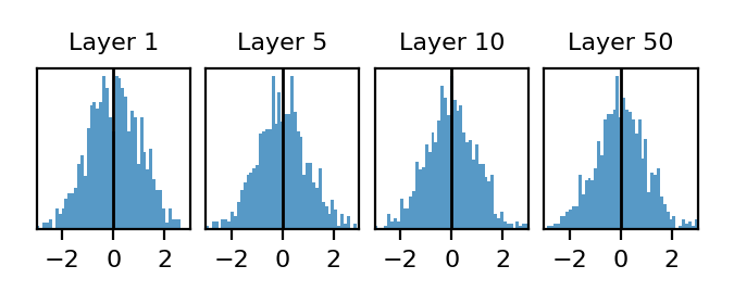
Ok, these distributions are boring. We just see a unit Gaussian at each layer. But it’s good that this is boring; Kaiming initialization is supposed to preserve the variance of each of these distributions.
Before moving on, let’s highlight some properties of preactivation distributions due to network randomness in a Kaiming-initialized ReLU network. These might seem simple, but only the fourth property will be true of distributions due to sample randomness so this stuff is actually pretty subtle.
Notationally, we will indicate averages over the network distribution with double brackets:
\[\llangle y \rrangle = \int y \; P(y | \mathbf{x}_0 ) \; d\mathbf{W}_1 d\mathbf{W}_2 ... d\mathbf{W}_L\]1. Every preactivation in the same layer has the same distribution
To see this theoretically, recall the relationship $\mathbf{y}_l = \mathbf{W}_l \mathbf{x}_{l-1}$. Because every element of $\mathbf{W}_l$ has the same distribution and is independent of $\mathbf{x}_l$, we have that every element of $\mathbf{y}_l$ has the same distribution.
2. Preactivations in every layer are zero mean
Again, this follows from the relationship $\mathbf{y}_{l} = \mathbf{W}_{l} \mathbf{x}_{l-1}$. Because $\mathbf{W}_l$ is independent of $\mathbf{x}_{l-1}$ and zero mean, we have that every element of $\mathbf{y}_{l}$ is zero mean: $\llangle y_l \rrangle = 0$.
3. Preactivations in every layer have the same variance
This is the statement that Kaiming initialization preserves neuron variance due to network randomness. I’ll provide a brief review of the argument they derived in their paper
Because elements of $\mathbf{W}_l$ have iid distributions over weights and elements of $\mathbf{y}_{l-1}$ are independent of $\mathbf{W}_l$, we can write the variance of an element of $\mathbf{y}_l$ as $\llangle y_l^2 \rrangle = N \; \llangle W_l^2 \rrangle \llangle f(y_{l-1})^2 \rrangle = 2 \llangle f(y_{l-1})^2 \rrangle$.
Over weights, elements of $\mathbf{y}_{l-1}$ are symmetrically distributed around zero. This implies that the 2nd moment of $\text{ReLU}$ of $\mathbf{y}_l$ is just half the 2nd moment of $\mathbf{y}_l$: $\llangle f(y_{l-1})^2 \rrangle = \frac{1}{2} \llangle y_{l-1}^2 \rrangle$.
The result:
\[\llangle y_l^2 \rrangle = \llangle y_{l-1}^2 \rrangle\]The variance over networks of a preactivation in layer $l$ is the same as it is in layer $l-1$ and therefore it is the same in every layaer. Note that if the weight variance were larger, variance of preactivations would grow exponentially, and if the weight variance were smaller, the pre-activation variance would decay exponentially.
4. Preactivations have Gaussian distributions if the network is infinitely wide.
Actually proving this is non-trivial. For empirical confirmation, just look at distributions we plotted above in our 1024 neuron wide network and observe that at least up to layer 50, they appear Gaussian.
We might think that regardless of network width, because $\mathbf{y}=\mathbf{W}_{l} \mathbf{x}_{l-1}$, each $y_i$ would be the sum $N$ Gaussian random variables $\sum_{j=1}^N W_{ij} x_j$ and would therefore be Gaussian. Certainly the $W$ have Gaussian distributions however the $x_j$ are complicated functions of the $W$ in previous layers and they generally are not Gaussian.
Even worse however, the $x_j$ are not independent random variables over weight configurations so we can’t even apply the central limit theorem to argue that $\sum_{j=1}^N W_{ij} x_j$ tends towards a Gaussian as the network width $N$ tends towards infinity.
The classic physics-style argument is to simply cheat and just treat the $x_j$ as though they are independent, then in the limit of large $N$ the sum $\sum_{j=1}^N W_{ij} x_j$ tends towards a Gaussian. This is called a mean-field approximation.
Layer Randomness
Before moving to examine distributions due sample randomness, we’ll examine another distribution which also arises from randomness in weight, but is much more convenient for the practitioner to actually measure. I am talking about layer randomness. This is the distribution of a neuron due to randomness in a single layer’s weights, with all other weights fixed:
\[P(y_l | \mathbf{x}_0, \mathbf{W}_1, \mathbf{W}_2, ..., \mathbf{W}_{l-1} ) \qquad \mathbf{W}_l \sim \mathcal{N}(0, 2/N)\]To visualize this distribution, we can sample a single fixed network (instead of 1000 like we did before) and now visualize the distribution of all preactivations in a layer:
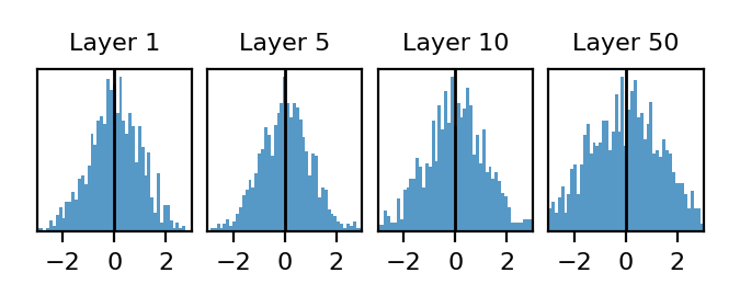
These look similar to the distributions due to network randomness (though there are some finite width effects that start to show up by layer 50). So long as the network is sufficiently wide, these distributions will be nearly identical to the distributions in the previous section that we got by allowing weight in every layer to fluctuate.
In the rest of this post, we will ignore any subtle differences between network and layer randomness and just focus on the difference between network and sample randomness.
Sample Randomness
Now things will get interesting (and more complicated). We’ll visualize a preactivation’s distribution due to sample randomness:
\[P(y_l | \mathbf{W}_1, \mathbf{W}_2, ..., \mathbf{W}_{l} ) \qquad \mathbf{x}_0 \sim Q(\mathbf{x}_0)\]This distribution is now a function of both the sample distribution $Q$ and the weights $\mathbf{W}_1, \mathbf{W}_2, …, \mathbf{W}_{l}$ in all layers up to layer $l$.
This distribution can be defined not just for random networks, but trained networks too. By carefully choosing the weights we can make this distribution look essentially any way we want, in fact the whole point of backprop-based training is make the network outputs have some desired distribution.
However, if we look at the “typical” behavior of this distribution in our ensemble of networks with Gaussian weights, we’ll see that it tends to take on certain regular properties, which we’ll describe below.
To visualize a typical sample distribution in a Kaiming-initialized network, we generate a single network with Kaiming initialization, and this time generate 1000 different input samples. For simplicity, we’ll choose use Gaussian white noise inputs:
\[Q = \mathcal{N} (0, I)\]We’ll visualize the empirical distribution over samples of a neuron in layers 1,5,10,50. To show that these distributions depend on the weights in a non-trivial way, we’ll repeat this process 3 times to get 3 different distributions in each layer. Each color corresponds to a network initialized with a different random seed.
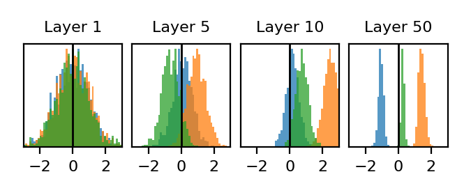
Completely different from the network randomness setting! Interestingly it appears that as we look deeper and deeper in the network, the distribution of each preactivation collapses to small fluctuations around some large mean value. The location of the mean value however, seems to depend on choice of random seed.
Instead of visualizing the sample distribution of a single neuron in each layer, we visualize the the distribution of all neurons over samples, i.e. we can visualize:
\[P(y_l | \mathbf{W}_1, \mathbf{W}_2, ..., \mathbf{W}_{l-1} ) \qquad \mathbf{x}_0 \sim Q(\mathbf{x}_0) \qquad \mathbf{W}_{l} \sim \mathcal{N}(0, 2/N)\]I show these histograms as red curves overlayed on top of the 3 previous single neuron histograms.
These histograms look more similar to the distributions arising from network or layer randomness, just zero mean Gaussian of constant width in each layer. These distributions are now arising from both layer and sample randomness. You dont’ see the interesting behavior if you average over weights.
With just an experiment, we can see that even in this extremely simple setup, preactivations can have very different distributions over weights vs. over samples.
With two approximations, we will actually be able to analytically describe the behavior of the mean and variance of preactivations over samples.
Network Averages and Sample Averages
Ultimately we will try to describe the behavior of the sample distribution via its mean and variance. As there are two sources of randomness, we have to be careful about which one we are averaging over.
Recall that we indicate averages due to randomness in weights in every layer with double brackets:
\[\llangle y \rrangle = \int y \; P(y | \mathbf{x}_0 ) \; d\mathbf{W}_1 d\mathbf{W}_2 ... d\mathbf{W}_L\]We will indicate averages due to sample randomness with single brackets:
\[\langle y \rangle = \int y \; P(y | \mathbf{W}_1 \mathbf{W}_2 ... \mathbf{W}_L ) \; d\mathbf{x}_0\]Note that the network mean $\llangle y \rrangle$ is as function of the input $\mathbf{x}_0$ and the sample mean $\langle y \rangle$ is a function of the network weights. We can also average over both sources of randomness, in which case the order does not matter:
\[\llangle \langle y \rangle \rrangle = \langle \llangle y \rrangle \rangle\]We have seen that for any particular input, the network average of every preactivation $\llangle y \rrangle$ is zero and the network variance $\llangle y^2 \rrangle - \llangle y \rrangle^2$ is the same in every layer. Intuitively, it might seem natural to compute the sample mean $\langle y \rangle$ and the sample variance $\langle y^2 \rangle - \langle y \rangle^2$ for some fixed set of weights.
Unfortunately this is not so simple. Each random seed used to initialize our networks resulted in a very different sample mean for each neuron. The distribution of sample means appeared to be centered around zero but each sample mean was quite different in each random network.
So rather than calculate the sample mean of a neuron for a single network, we will try to describe its typical behavior in the ensemble of random networks defined by random Gaussian weights.
Specifically we will calculate the network variance of the sample mean:
\[m^2 = \llangle \langle y \rangle^2 \rrangle - \llangle \langle y \rangle \rrangle^2 = \llangle \langle y \rangle^2 \rrangle\]and the average of the sample variance over network configurations:
\[v^2 = \llangle \langle y^2 \rangle - \langle y \rangle^2 \rrangle\]The two are related, in fact the sum of $m^2$ and $v^2$ is just the total variance of a neuron; i.e. the variance due to randomness in both weights and samples:
\[\sigma^2 = \llangle \langle y^2 \rangle \rrangle = m^2 + v^2\]Basically, due to randomness in the weights, each neuron exhibits fluctuations both in the location of its sample mean and fluctuations around the mean. If you compute the variance over weights of a preactivation, you are potentially “overestimating” the sample variance of any neuron in a fixed network as there is a contribution from fluctuations in the location of the neuron’s mean. Let’s see how this all works out.
Analytic behavior of sample mean and variance
To analytically compute $m_l^2$ and $v_l^2$, we will assume our network is infinitely wide and make 2 mean-field approximations that will be allow us to assume Gaussian distributions.
Mean-field Approximations:
One, we make make a mean-field approximation over weights. This means we assume that for any fixed input, we treat the activations $x_i$ as independent random variables over weight randomness.
Two, make a mean-field approximation over samples. This means we assume that for any fixed network configuration, we treat the activations $x_i$ as independent random variables over sample randomness.
Now we will be ready to describe the behavior of the typical sample mean and variance.
Property 1: Within a layer, the sample variance of every preactivation is the same:
\[\langle y_l^2 \rangle - \langle y_l \rangle^2 \approx \llangle \langle y_l^2 \rangle - \langle y_l \rangle^2 \rrangle = v_l^2\]In the language of physicists we would say that the variance of $y$ is a self-averaging quantity because it is the same over (almost) all weight configurations.
This is actually a pretty subtle point. For instance neither $\langle y_l^2 \rangle$ nor $\langle y_l \rangle^2$ are self-averaging, only their difference is. Additionally, the sample variance of activations is not self-averaging, only the sample variance of activations. Unfortunately I don’t have an intuitive explanation for this. So I moved the justification to the end of this blog post. Check it out at your own peril.
Property 2: A preactivation’s distribution over samples is Gaussian:
\[y_l ~ \sim \mathcal{N}(\langle y_l \rangle, v_l^2)\]With the mean-field approximation over samples and the relationship $y_i = \sum_j W_{ij} x_j$, we can see that $y$ is the sum of $N$ independent random variables. Since we have assumed an infinitely wide net, $y$ will tend towards a gaussian as a consequence of the central limit theorem.
Property 3: A preactivation’s sample mean has a Gaussian distribution over networks configurations:
\[\langle y_l \rangle \sim \mathcal{N}(0, m_l^2)\]This is a consequence of the mean-field approximation over weights. Using the relationship $y_i = \sum_j W_{ij} x_j$ we can see that the sample mean is the sum of $N$ random variables: $\langle y_i \rangle = \sum_j W_{ij} \langle x_j \rangle$. Since we assume the $x_j$ are independent, $\langle y \rangle$ will tend towards a gaussian as a consequence of the central limit theorem.
Property 4: $m,v,\sigma$ are described by the following layerwise trajectory:

The sample standard deviation $v_l$ decays to zero (slowly) with increasing layer and the expected squared sample mean $m_l$ approaches the total standard deviation $\sigma_l$ with increasing layer. Intuitively this means that input samples get mapped to small fluctuations around increasingly large sample-independent mean values in each layer. This is exactly what we saw in our experiments.
Formally, the ratio $r_l = m_l/v_l$ can be described by the iterated map:
\[r_{l+1}^2 = r_l \left[ 1 + \frac{1}{\pi} \left(\sqrt{1/c^2 - 1} - \cos^{-1}(c)) \right) \right]\]where $c^2 = \frac{r^2}{1+r^2}$.
We can use the fact that $m_l^2 + v_l^2 = \sigma_l^2$ and the fact that the total variance is preserved ($\sigma_{l+1}^2 = \sigma_l^2$) to generate the above curves.
Derivation:
First we’ll relate the expected squared sample mean of an element of $\mathbf{y}_{l+1}$ to the expected squared sample mean of an element of $f(\mathbf{y}_l)$. This is simple enough to do by using the relationship $\mathbf{y}_{l+1} = \mathbf{W}_{l+1} f(\mathbf{y}_l)$. The result:
\[m_{l+1}^2 = \llangle \langle y_{l+1} \rangle^2 \rrangle = 2 \llangle \langle f(y_{l}) \rangle^2 \rrangle\]Now we want to relate the expected squared sample mean of an element of an element of $\mathbf{y}_{l}$ to the expected squared sample mean of an element of an element of $f(\mathbf{y}_l)$. This one is trickier.
Let’s assume we know the sample mean of a preactivation in layer $l$. For notational convenience, we’ll decompose every preactivation into the sum of its sample mean $\mu_l$ and fluctuations around the mean $\nu_l$:
\[y_l = \mu_l + \nu_l\]Using approximation 1 that the sample variance of this preactivation is $v_l^2$ and approximation 2 that the distribution of this preactivation is just a Gaussian centered at $\mu$ and variance $v_l^2$, we can compute the sample variance of the subsequent activation:
\[\langle f(y_{l}) \rangle = \int f(\mu + \nu) P(\nu) d\nu \qquad P(\nu) = \mathcal{N}(0, v_l^2)\]Now we use approximation 3 that the sample mean $\mu_l$ has a Gaussian distribution with variance $m_l^2$ to compute the expected squared sample mean of the activation:
\[\llangle \langle f(y_{l}) \rangle^2 \rrangle = \int \left[\int f(\mu + \nu) P(\nu) d\nu\right]^2 P(\mu) d\mu\]Ok, this might seem a little ugly at this point, but it turns out this integral has been studied before, notably by Cho and Saul. It is closely related to the arccosine kernel and can be analytically evaluated as a function of $m^l$ and $v^l$. Evaluating the integral and using the relationship that $m_{l+1}^2 =2 \llangle \langle f(y_{l}) \rangle^2 \rrangle$ we get:
\[m_{l+1}^2 = m_l^2 \left[ 1 + \frac{1}{\pi} \left(\sqrt{1/c_l^2 - 1} - \cos^{-1}(c_l)) \right) \right]\]where $c_l^2 = \frac{m_l^2}{m_l^2+v_l^2}$.
It’s not pretty but its exact. Let’s note one thing before moving on. In some sense, the integral only depends in an interesting way on the ratio $m_l/v_l$ (all the interesting stuff is a function of $c$ which is only a function of the ratio of $m/v$).
This makes sense, both matrix multiplication and the $\text{ReLU}$ nonlinearity are scale-free. Doubling the input simply doubles the output. This scale shows up in the prefactor of $m$.
As an exercise, it might be worth using this integral approach to confirm that $\sigma_{l+1}^2 = \sigma_{l}^2$. This would be rederiving the result that Kaiming initialization preserves the total variance.
Empirical Check
We can empirically confirm our results. We simply initialize the same fully connected network we studied before and pass in a bunch of Gaussian white noise and calculate the ratio of the sample mean to standard deviation at each layer. We’ll do this several times and for several different network widths. This figure is taken from our paper
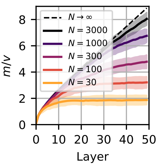
The dashed line is what we get with our preceding calculation. The solid lines indicate the average ratio over network instantiations and the shaded regions show the standard deviation over instantiations. As we increase the width our calculation becomes more and more accurate. Great!
Justification for Self-Averaging Variance
In our calculation, we assumed that the sample variance of every preactivation is this same. We said this is a consequence of the mean-field approximation over samples and the wide network limit. Now its time to show this.
We show that the sample variance is self-averaging is by directly computing the network variance of the sample variance and showing that it is small.
\[\llangle v^4 \rrangle - \llangle v^2 \rrangle^2 = \llangle (\langle y^2 \rangle - \langle y \rangle^2)^2 \rrangle - \llangle \langle y^2 \rangle - \langle y \rangle^2 \rrangle^2\]With the relationship $\mathbf{y} = \mathbf{W} \mathbf{x}$ we can relate this to the covariance matrix of activations, $C = \langle \mathbf{x} \mathbf{x}^{\top} \rangle - \langle \mathbf{x} \rangle \langle \mathbf{x} \rangle^{\top}$, in the previous layer:
\[\llangle v^4 \rrangle - \llangle v^2 \rrangle^2 =\llangle \text{Tr}[ \mathbf{W} \mathbf{C} \mathbf{W}^{\top} \mathbf{W} \mathbf{C} \mathbf{W}^{\top} ] \rrangle\]Yikes… But with some properties of random matrices (and painful arithmetic), we can relate this to expected eigenvalues of the activation covariance matrix:
\[\llangle v^4 \rrangle - \llangle v^2 \rrangle^2 = \frac{1}{N} \left[\llangle \lambda^2 \rrangle - \llangle \lambda \rrangle^2\right]\]Great, we have a factor $\frac{1}{N}$. Doesn’t this suggest that so long as the network is infinitely wide the fluctuations of the sample variance go to zero? Not quite. Unfortunately the eigenvalues might also scale with $N$.
Here is where we use the mean field approximation. If we pretend all the activations are independent over samples, then basically there are no strong correlations and the covariance matrix has a relatively “flat” power spectrum: all eigenvalues are the same. This implies that the average square eigenvalue of the covariance matrix $\llangle \lambda^2 \rrangle$ is roughly just the square of the average $\llangle \lambda^2 \rrangle$.
Why doesn’t this work if we instead computed the preactivation 2nd moment, rather than the variance? If we went back through the argument, we’d find that the variance instead depends on the first and second moment of eigenvalues of the correlation matrix: $C = \langle \mathbf{x} \mathbf{x}^{\top} \rangle$.
Even if all the activations are independent, they may still have some finite mean value. In this case, the spectrum of this corelation matrix will relatively flat except for 1 order N eigenvalue. In this scenario the 2nd moment $\llangle \lambda^2 \rrangle$ will also be $O(N)$ while the 1st moment $\llangle \lambda \rrangle$ will be $O(1)$. The difference will be $O(N)$ and so the network variance of the sample variance will be non-zero: it exhibits large fluctuations over network configurations.
Discussion
So apparently the statement “Kaiming initialization preserves variance” is actually pretty subtle. Its true if you compute the variance over weight randomness. But the variance over samples, arguably the more relevant quantity in practical deep learning, actually decays with depth!
Batch/Layer/Group Normalization
Typically, people think of normalization schemes as ways to “reduce covariate shift, smooth loss surface, etc” but we can use our theory to understand how popular normalization schemes actually alter the initialization of a network.
Standard normalization schemes normalize preactivations:
\[y \leftarrow \frac{y - \mu}{ \sigma }\]Batch Normalization uses the minibatch mean and minibatch variance. When your minibatch is large, these will be closely related to the sample mean, and sample variance. This implies that every preactivation will be zero mean and unit variance, a big difference from the unnormalized case!
Layer Normalization uses the layer mean and layer variance, which we’ve argued are closely related to network mean and variance. So this might not have such a big effect, at least in the wide network case. Is this a possible source of the discrepancy in training between layer and batch norm?
Group Normalization is something like a mix between the Batch and Layer Normalization. It normalizes with the mean and variance over subsets of neurons in a layer.
Implications for Training
The real question is “does any of this matter for training?” My answer is definitely YES, IT CAN MATTER. In fact the whole reason I wrote this post was that while experimenting with various initializations for training UNets, I observed that normalizing pre-activations with the mean and standard deviation computed over samples (similar to Batch Norm) seemed to provide a noticeable speedup to training compared to when i used the values computed over a layer.
This originally confused me, as I incorrectly thought the two statistics would be similar. In our paper, we also trained a 10 layer “All Convolutional Net” and found that normalizing with the sample statistics at initialization outperformed normalization with layer statistics.
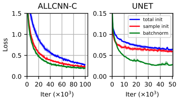
Interestingly, just reinitializing seemed to provide a substantial fractino of the speedup provided by Batch Norm.
Now, for the question of does it always matter, and when does it matter? I’m less sure about to this. It seems like sometimes reinitializing is not always helpful. Check out David Page’s post for some info!
Relation to Signal Propagation Formalism
Starting with Poole et al., a number of works have considered how the correlation between preactivations from two different inputs
\[c_{ab} = \llangle y_a y_b \rrangle\]propagates through layers of a network.
They identify two key behaviors in random networks. In the “chaotic regime”, inputs with high correlation (very similar inputs) get mapped to very small correlations (very dissimilar activations) in higher layers. In the “ordered regime”, inputs with high correlation (very similar inputs) get mapped to even higher correlations (more similiar activations) in higher layers.
How does this relate to sample statistics? The expected squared sample mean is simply the average of this quantity over independently chosen pairs of inputs:
\[\langle c_{ab} \rangle = \langle \llangle y_a y_b \rrangle \rangle = \llangle \langle y \rangle^2 \rrangle = m^2\]Why is this interesting? One, when inputs get mapped to more similar acitvation patterns, the sample mean of preactivations increases at each layer. Perhaps more interestingly, any time the mean of preactivations is zero (such as in Batch Normalized networks), there is no possibility that the network is in the ordered regime (otherwise the mean would increase in each layer).
Acknowledgements
The post originated from work done with my advisor Sebastian Seung.