Why Batch Norm Causes Exploding Gradients

$$ \def\llangle{\langle \! \langle} \def\rrangle{\rangle \! \rangle} \def\lllangle{\left \langle \!\! \left \langle} \def\rrrangle{\right \rangle \!\! \right \rangle} $$

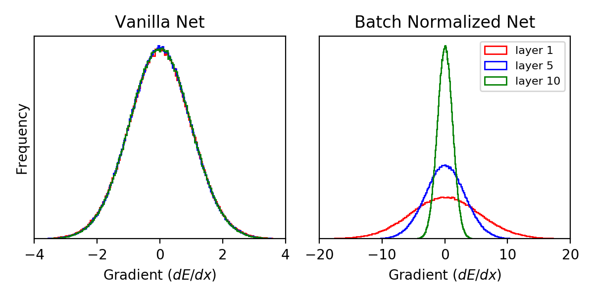
Gradient histograms in a 10 layer network at initialization. The typical size of gradients is the same in all layers in a net without Batch Norm (left) and grows exponentially after inserting Batch Norm in every layer (right)

Deep learning practitioners know that using Batch Norm generally makes it easier to train deep networks. They also know that the presence of exploding gradients generally makes it harder to train deep networks. So recent work by Yang et. al might seem quite surprising; they show that our beloved Batch Norm can actually cause exploding gradients, at least at initialization time.

I like their paper because it has the rare quality of saying something both rigorous and meaningful about Batch Norm. Unfortunately, there’s not much intuition behind the 95 pages of technical mathematics comprising the paper. In this post I’ll provide a more intuitive explanation for the gradient explosion phenomenon. With a few “back-of-the-envelope” calculations (and admittedly a big envelope), we can show in simplified settings that gradient norms grow by $\sqrt{\pi/(\pi-1)}$ in each layer of a ReLU network with Batch Normalization.

TL;DR Inserting Batch Norm into a network means that in the forward pass each neuron is divided by its standard deviation, $\sigma$, computed over a minibatch of samples. In the backward pass, gradients are divided by the same $\sigma$. In ReLU nets, we’ll show that this standard deviation is less than 1, in fact we can approximate $\sigma\approx \sqrt{(\pi-1)/ \pi} \approx 0.82$. Since this occurs at every layer, gradient norms in early layers are amplified by roughly $1.21 \approx (1/0.82)$ in every layer.

What are “exploding gradients”?

Before our calculation, let’s empirically show that “Batch Norm causes exploding gradients”. We’ll just initialize a net without Batchnorm, compute gradients, then insert Batch Norm into every layer of the net and recompute gradients and see how they differ.

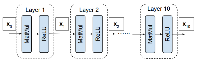
Our net without Batch Norm, our “vanilla net”, is shown below. Its a boring old 10 layer, feedforward, fully connected network of uniform layer width $N=1024$. We’re using the ReLU nonlinearity so we’ll initialize weights with Kaiming initialization. This means we’ll set all the biases to zero and sample every element of $W$ from a zero mean Gaussian with variance $\sqrt{2/N}$.

Our inputs $\mathbf{x}_0(t)$ are 512 random Gaussian vectors. We’ll compute a linear loss over the network’s outputs: $E = \sum_{t=1}^{512} \mathbf{w} \cdot \mathbf{x}_{10}(t)$. We choose $\mathbf{w}$ by drawing it from a unit Gaussian. Now we have everything we need to compute the gradients $dE/d\mathbf{x}_l(t)$ at each layer $l$ in the vanilla network (We’ll use Pytorch to automate this process for us).

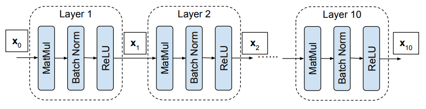
Now we take that exact network, loss, and set of input vectors, but insert Batch Normalization before the ReLU in every layer:

Again we can compute gradients $dE/d\mathbf{x}_l(t)$ at each layer. Now we’ll visualize the gradient histograms in each layer for the vanilla and Batch Norm net. Each histogram is made up of $512\times1024$ scalars (gradients for 512 inputs $\times$ 1024 features):

In the vanilla network, the gradient histograms are basically the same in every layer. However, after inserting Batch Norm, the gradients actually grow with decreasing layer. In fact, the widths of these histograms grow exponentially. It is in this sense that gradients explode. The rest of this post will be devoted to calculating how the widths of these histograms grow.

Gradients in a Batch Normalized Net

In this section we’ll review the details of Batch Normalization and how it modifies the forward and backward pass of a neural network.

Forward Pass

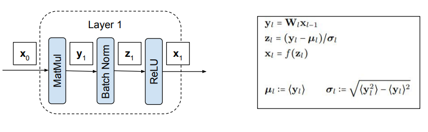
Each layer in our normalized network contains 3 modules: matrix multiply, Batch Norm, and ReLU. These are shown in the diagram above.

$\mathbf{x}_l, \mathbf{y}_l$ and $\mathbf{z}_l$ denote the vector outputs of the matrix multiply, Batch Norm, and ReLU modules in layer $l$ for a single input. The element-wise product is denoted by $\mathbf{a} \circ \mathbf{b}$. We’ll abuse notation and denote element-wise division with $\mathbf{a}/\mathbf{b}$. The notation $\langle \cdot \rangle$ indicates a minibatch average so $\boldsymbol{\mu}_l$ and $\boldsymbol{\sigma}^2_l$ are the mean and variance of each element of $\mathbf{y}_l$ over a minibatch. $f$ is the ReLU nonlinearity which acts element-wise on an input vector.

Because we are only going to examine networks at initializion time, we have made two simplifications. One, we ignore bias addition in the matrix multiply layer as biases are initialized to zero. Two, we can ignore the part of Batch Norm with learnable parameters which transforms $\mathbf{z}_l \leftarrow \boldsymbol{\gamma}_l \circ \mathbf{z}_l + \boldsymbol{\beta}_l$ because $\boldsymbol{\gamma}_l=\boldsymbol{1}$ and $\boldsymbol{\beta}_l=\boldsymbol{0}$ at initialization.

Backward Pass

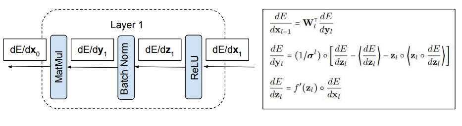
The diagram above shows the backwards pass through each module. Recall that the backwards pass applies the chain rule to compute gradients with respect to a module’s inputs, given gradients with respect to the module’s outputs.

For the Batch Norm module this gets rather tedious. Fortunately this is derived in the original Batch Norm paper, which I have simplified in the diagram above. If you want a step-by-step derivation, check out this blog post!

Before moving on, we’ll highlight two superficial similarities between the forwards and backwards pass through a Batch Norm module. One, division by $\boldsymbol{\sigma}_l$ occurs in each case. Two, in the same way Batch Norm centers the forwards pass, $\langle \mathbf{z}_l \rangle = \boldsymbol{0}$, it also centers gradients in the backwards pass, $\langle \frac{dE}{d\mathbf{y}} \rangle = \boldsymbol{0}$.

Typical Gradients in a Batch Normalized Net

Our goal was to understand how the width of the gradient histogram grows at each layer in our experiment. Recall that each histogram contained the gradient of every neuron in a layer computed over all samples. Since this histogram is zero-mean, we can easily compute this width in our experiment: $\frac{1}{T}\sum_{t=1}^{T} \frac{1}{N}\sum_{i=1}^{N} \left(\frac{dE}{dx_{l,i}(t)}\right)^2$.

However, we want to understand theoretically how this width grows, and this sum is not particularly enlightening. Since $N$ is large in our experiments, the unwieldy sum over neurons is a decent approximation for a much simpler quantity: the squared gradient of a single neuron, averaged over weights.

\[\text{Typical Squared Gradient } = \lllangle \left( \frac{dE}{dx_l(t)}\right)^2 \rrrangle \approx \frac{1}{N}\sum_{i=1}^N \left(\frac{dE}{dx_{l,i}(t)}\right)^2\]

The double brackets $\llangle \cdot \rrangle$ indicate an average over weights in all layers. Also note that we have dropped the index $i$ on the left side of the equation, it is is the same for every neuron in a layer (because the weights have identical distributions). So the histogram width is nearly equal to the typical squared gradient, averaged over samples in the minibatch.

To compute the typical squared gradient, we just need to square and average over weights each backwards pass equation for the three modules comprising each layer. Before deriving these, I’ll just show the results:

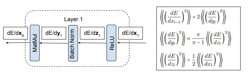
The ReLU module halves the average squared gradients and the matrix multiply module doubles the average squared gradient. So the combination preserves average squared gradients. In fact this was part of the original motivation given in the Kaiming initialization paper; set the weight variance to $2/N$ so gradients are preserved in networks without Batch Norm.

The interesting thing happens in the Batch Norm module. It amplifies average squared gradients by $\pi/(\pi-1)$. Note the approximation sign here. To calculate this we assume we have a wide network and a large minibatch with “sufficient randomness”.

Now let’s get to the derivation. Computing the typical squared backward pass through the matrix multiply and ReLU modules has been done before and is not so complicated, so we’ll move quickly to get the final results. If you want a more in depth derivation, check out either the Kaiming initialization paper or this blog post!

Matrix Multiply Module

Consider the backwards pass through a matrix multiply module $\frac{dE}{dx_i} = \sum_{j} W_{ji} \frac{dE}{dy_j}$. To minimize clutter, we’ve removed layer indices $l-1,l$ on the $x,y,W$. Now lets derive the “typical backpropagation” equation.

Step 1: Square both sides and average over weight configurations:

\[\lllangle \left(\frac{dE}{dx_i}\right)^2 \rrrangle = \sum_{jk} \lllangle W_{ji} W_{ki} \frac{dE}{dy_j} \frac{dE}{dy_k} \rrrangle\]

Step 2: To make further progress, we need to assume that forward pass quantities are independent from backwards pass quantities, over randomness in the weights. This is called the “gradient independence” assumption. This allows us to separate the $W$ terms and $dE/dy$ terms:

\[\lllangle \left(\frac{dE}{dx_i}\right)^2 \rrrangle = \sum_{jk} \llangle W_{ji} W_{ki} \rrangle \lllangle \frac{dE}{dy_j} \frac{dE}{dy_k} \rrrangle\]

Step 3: We can simplify the sum using the fact that $W_{ij}$ are independent zero mean variables with variance $2/N$ so $\llangle W_{ji} W_{ki} \rrangle = (2/N)$ if $j=k$ and 0 otherwise

\[\lllangle \left(\frac{dE}{dx_i}\right)^2 \rrrangle = (2/N) \sum_{j} \lllangle \left(\frac{dE}{dy_j}\right)^2 \rrrangle\]

Step 4: Use the fact that the typical squared gradient at each layer is the same for all elements. This follows from the identical distribution of $W$.

\[\boxed{ \lllangle \left(\frac{dE}{dx_{l-1}}\right)^2 \rrrangle = 2 \lllangle \left(\frac{dE}{dy_l}\right)^2 \rrrangle }\]

ReLU Module

Consider the backwards pass through the ReLU module $\frac{dE}{dz_i} = f’(z_i) \frac{dE}{dx_i}$. Let’s procede like before.

Step 1: Square both sides of the backward pass equation and average over weights:

\[\lllangle \left(\frac{dE}{dz_i}\right)^2 \rrrangle = \lllangle f'(z_i)^2 \left( \frac{dE}{dx_i} \right)^2 \rrrangle\]

Step 2: Separate the $f’$ terms and $dE/dx$ terms using the gradient independence assumption:

\[\lllangle \left(\frac{dE}{dz_i}\right)^2 \rrrangle = \llangle f'(z_i)^2 \rrangle \lllangle \left( \frac{dE}{dx_i} \right)^2 \rrrangle\]

Step 3: ReLU is a particularly simple activation. If $z_i > 0$, then $f’ = 1$. Otherwise $f’=0$. This is great, since over weight configurations $z_i>0$ half the time and $z_i < 0$ the other half. So the average $\llangle f’(z_i)^2 \rrangle = 1/2$:

\[\boxed{ \lllangle \left(\frac{dE}{dz}\right)^2 \rrrangle = \frac{1}{2} \lllangle \left( \frac{dE}{dx} \right)^2 \rrrangle }\]

At this point, we can combine the typical backwards pass equations for the ReLU and the matrix multiply module to see that if we didn’t have Batch Norm, gradients would preserved

\[\lllangle \left(\frac{dE}{dx_{l-1}}\right)^2 \rrrangle = \lllangle \left( \frac{dE}{dx_{l}} \right)^2 \rrrangle\]

Batch Norm Module

In some sense, 2/3 of our work is done; in principle we just need to average the squared backwards pass equations over weights like we did before. However in a much more real sense, most of the work is still to come.

The first complication is the gradients that come from backpropagating through the minibatch mean $\mu$ and variance $\sigma^2$. We will argue that these gradients are nearly zero, at least if there is enough “randomness” in the data and the networks are sufficiently wide.

The second complication is the division by $\sigma$, the minibatch standard deviation. Since it is an average over samples, not weights, it will take some assumptions (and labor) to calculate.

Approximation 1: $\langle z \frac{dE}{dz} \rangle \approx 0$

We are going to argue that $\langle z \frac{dE}{dz} \rangle$, the term from backpropagating through $\sigma$, is nearly zero at initialization time.

To do so we’ll extend the gradient independence assumption to apply over the minibatch distribution. This means that for a typical configuration of weights, we assume forward pass quantities are independent from backward pass quantities over the minibatch distribution¹.

With this assumption we have

\[\langle \mathbf{z} \circ \frac{dE}{d\mathbf{z}} \rangle \approx \langle \mathbf{z} \rangle \circ \langle \frac{dE}{d\mathbf{z}} \rangle = \mathbf{0}\]

The last equality follows from the fact that $\langle \mathbf{z} \rangle = \mathbf{0}$ because Batch Norm explicitly centers this variable.

Approximation 2: $\langle \frac{dE}{dz} \rangle \approx 0$

Now we’ll argue that $\langle \frac{dE}{dz} \rangle$, the term from backpropagating through $\mu$, is nearly zero at initialization time, except possibly in the last layer.

First note that Batch Norm ensures gradients with respect to $\mathbf{y}$ are exactly zero mean: $\langle \frac{dE}{d\mathbf{y}} \rangle = \mathbf{0}$.With our backwards pass equations, we can write gradients for $\mathbf{z}_l$ in terms of gradients for $\mathbf{y}_{l+1}$: $\frac{dE}{d\mathbf{z_l}} = f’(\mathbf{z_l}) \circ \mathbf{W}_l^T \frac{dE} {d\mathbf{y}_{l+1}}$.

Now we average both sides of this equation over samples in the minibatch. With the extended gradient independence assumption, $f’(\mathbf{z_l})$ and $\frac{dE} {d\mathbf{y}_{l+1}}$ are independent quantities so we can simplify the minibatch-averaged sum:

\[\left\langle \frac{dE}{d\mathbf{z}_l} \right\rangle \approx \langle f'(\mathbf{z}_l) \rangle \circ \mathbf{W}_l^T \left\langle \frac{dE} {d\mathbf{y}_{l+1}} \right\rangle = 0\]

Note that this argument doesn’t really hold up in the last layer; we required a Batch Norm in layer $l+1$ to center incoming gradients to layer $l$. So if there are only $L$ layers in the network, gradient signals to $\mathbf{z}_L$ might not be centered. But we won’t get too worked up if this doesnt hold for just one layer.

Combining the last two approximations, we are left with the greatly simplified backwards pass equation:

\[\frac{dE}{d\mathbf{y}_l} \approx \frac{1}{\boldsymbol{\sigma}_l} \circ \frac{dE}{d\mathbf{z}_l}\]

The next step will be to average this over weights like we did for the matrix multiply and ReLU modules.

Approximation 3: $\sigma^2 \approx \frac{\pi-1}{\pi}$

We’re in the home stretch. Squaring then averaging the final equation over weights gives us:

\[\lllangle \left(\frac{dE}{dy_{l}}\right)^2 \rrrangle \approx \lllangle \frac{1}{\sigma_l^2} \rrrangle \lllangle \left(\frac{dE}{dz_{l}}\right)^2 \rrrangle\]

All that remains is to compute $\llangle (1/\sigma_l)^2 \rrangle$, the expected inverse variance of an element of $\mathbf{y}_l$. While we already know that $\llangle (1/\sigma_l)^2 \rrangle \approx 1.2$ from our simulations (this is the factor by which the width of gradient histograms grew every layer), let’s calculate it analytically.

Step 1: Let’s start with something we do know the variance of. Because $z$ is the output of a Batch Norm module, it has to be zero-mean and unit variance over the minibatch. Since $x$ is just a rectified version of $z$, it might seem like we can relate the variance of $x$ to $z$.

Unfortunately knowing the mean and variance of $z$ is not enough to evaluate either of these integrals. It seems like a reasonable assumption however that $z$ will take a Gaussian distribution because $z$ is just a centered and scaled version of $y$, and $y$ is the sum of $N$ random variables. Also it’s easy enough to visualize histograms of $z$ in our experiment and confirm that it appears Gaussian.

Now we just have to integrate the unit Gaussian over the positive half:

\[\langle x^2 \rangle - \langle x \rangle^2 = \frac{1}{\sqrt{2\pi}} \int_{0}^{+\infty} z^2 e^{\frac{-z^2}{2}} dz - \left[\frac{1}{\sqrt{2\pi}} \int_{0}^{+\infty} z e^{\frac{-z^2}{2}} dz\right]^2\]

The first term is just $\frac{1}{2}$ (half the variance of a unit Gaussian). The 2nd term is $\frac{1}{2\pi}$ which follows from direct integration: $\int z e^{-z^2/2} dz = e^{-z^2/2}$.

Step 2: Now we can relate the expected variance of an element of $y$ to the variance of $x$ (recall that the minibatch variance is computed over samples in the minibatch, and in general it depends on the network weights):

\[\sigma^2 = \langle y^2 \rangle - \langle y \rangle^2 = \mathbf{w}^{\top} \left[ \langle \mathbf{x} \mathbf{x}^{\top} \rangle - \langle \mathbf{x} \rangle \langle \mathbf{x} \rangle^{\top} \right] \ \mathbf{w} = \mathbf{w}^{\top} \mathbf{C}^{xx} \mathbf{w}\]

It is simple enough to compute the average minibatch variance $\llangle \sigma^2 \rrangle$. When $i\neq j$ we have $\llangle w_i w_j \rrangle = 0$ and when $i=j$ we have $\llangle w_i w_j \rrangle = \sqrt{2}/N$. Since we have assumed the $x$ are identically distributed, we are left with the result:

\[\llangle \sigma^2 \rrangle = 2 \llangle \langle x^2 \rangle - \langle x \rangle^2 \rrangle = \frac{\pi-1}{\pi}\]

Step 3: We’ve computed $\llangle \sigma^2 \rrangle$, but this is generally different from $\llangle 1/\sigma^2 \rrangle$, which is the quantity we wanted. We’ll argue that in our experiment, these are actually the same because fluctuations of $\sigma^2$ are small so $\llangle \frac{1}{\sigma^2} \rrangle \approx \frac{1}{\llangle \sigma^2 \rrangle}$

In physics terms, we argue that $\sigma^2$, the minibatch variance of an element of $\mathbf{y}$, is a self-averaging quantity. This means that for nearly every configuration of weights, $\sigma^2$ is roughly the same²:

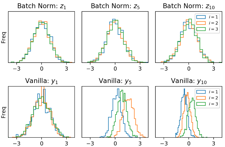
\[\langle y^2 \rangle - \langle y \rangle^2 \approx \llangle \langle y^2 \rangle - \langle y \rangle^2 \rrangle\]

We can empirically show this self-averaging assumption holds in our simulation. We’ll do so by visualizing the distribution of the first 3 elements of $\mathbf{y}$ in the 5th layer of our Batch Normalized net.

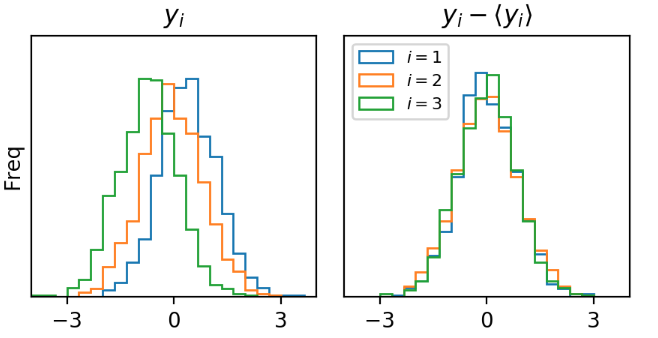
Interestingly each element of $\mathbf{y}$ seems to have a different mean, but we can see that fluctuations around the mean appear to have identical distributions. This means that the variance of every element is the same (roughly).

Step 4: We’ve made it to the end. We can combine our estimate $\llangle 1/\sigma^2\rrangle = \frac{\pi}{\pi-1}$ with our typical backward pass equation through a Batch Norm module: $\lllangle \left(\frac{dE}{dy_{l}}\right)^2 \rrrangle \approx \lllangle \frac{1}{\sigma_l^2} \rrrangle \lllangle \left(\frac{dE}{dz_{l}}\right)^2 \rrrangle$ to see how Batch Norm amplifies the gradients in the backwards pass:

\[\boxed{ \lllangle \left(\frac{dE}{dy_{l}}\right)^2 \rrrangle \approx \left(\frac{\pi}{\pi-1}\right) \lllangle \left(\frac{dE}{dz_{l}}\right)^2 \rrrangle }\]

Result: Squared Gradients Amplified by $\frac{\pi}{\pi-1}$

Combining the typical backwards pass equations through every layer, we get the final result that squared gradients are amplified by $\frac{\pi}{\pi-1}$ at every layer:

\[\lllangle \left(\frac{dE}{dx_{l-1}}\right)^2 \rrrangle \approx \left(\frac{\pi}{\pi-1}\right) \lllangle \left(\frac{dE}{dx_{l}}\right)^2 \rrrangle\]

Of course we can empirically test our approximations by measuring the width of the gradient histograms in each layer of our simulation:

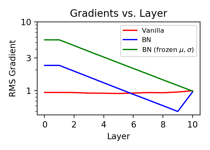
I also ran a 3rd experiment, this time freezing $\mu$ and $\sigma$. So the forward pass of this network was identical to the Batch Norm network, but gradients were not backpropagated through the $\mu$ and $\sigma$. Earlier we predicted that expect possibly in the final layer, gradient backpropagation probably wasn’t changed much by $\mu$ and $\sigma$ in a random network.

In both cases, I measured the the RMS gradient (the width of each histogram) to by 1.21, which as expected is very close to $\sqrt{\pi/(\pi-1)}$. Cool, the theory worked!

Normalized Preactivations Imply Very Nonlinear Input-Output Mappings

Before concluding, we’ll give one more way to think about the exploding gradient phenomenon: by normalizing the inputs to the ReLU nonlinearity, you are ensuring that the nonlinearity is used “more effectively” at each layer and the network is more likely to implement some crazy nonlinear function which massively distorts the geometry of the input space.

This probably makes more sense if we just look at the distribution of inputs to ReLU in the vanilla and normalized networks:

In deeper layers of the vanilla net, some of the preactivations lie mostly on one side of the nonlinearity. When this happens, the ReLU activation either computes the function $x_i=y_i$ for all inputs or it computes $x_i=0$ for all inputs; either way, it’s acting in a linear fashion. This does not happen in the normalized network because inputs to the ReLU are centered by Batch Norm

The authors of the original “Mean Field Theory of Batch Normalization” paper would say the network which normalizes preactivations and therefore implements a highly nonlinear function is in a state of transient chaos.

Does this matter for Real World Network Training?

I’m really not sure.

Maybe it doesn’t matter. One, the actual factor by which gradients explode, at least in our scenario, is not too extreme. They grow by 1.21 at each layer, even after 10 layers this means gradients are just 6x larger in the beginning. This is probably not a crippling difference. And this might be small compared to differences coming from variable layer widths, residual connections, and other complications in real world networks. Two, all this analysis was in random networks. Relating this to training dynamics is not a simple matter.

But maybe it does matter. The authors of the “Mean Field Theory of Batch Normalization” paper show that extremely deep feedforward nets (50+ layers) are hard or impossible to train with Batch Norm. One might object that the deepest real world networks aren’t just 50 layers of matrix multiplication or convolution stacked on top of each other, but they include residual connections too. Perhaps this is no coincidence, maybe Batch Norm is not helpful, or is even harmful in extremely deep nets without other tricks.

Acknowledgements

The post originated from work done with my advisor Sebastian Seung.

Footnotes

1. This assumption might seem a little odd; at some level deep learning only works because the gradients are functions of the parameters at each layer so they can tell us how to update the parameters to improve the loss. We are basically assuming there is enough “noise” in these gradients over the minibatch distribution. We are assuming that dependencies between forward pass quantities and backwards pass quantities are small compared to fluctuations in the values of forward pass and backwards pass quantities over the minibatch. (If you still don’t like this assumption we’ll later show empirically it seems to hold in our experiment). ↩

2. Actually we could theoretically show that $\sigma^2$ is self-averaging by showing that eigenvalues of the covariance matrix $\langle \mathbf{x} \mathbf{x}^{\top} \rangle - \langle \mathbf{x} \rangle \langle \mathbf{x} \rangle^{\top}$ are “well behaved” (meaning none of the eigenvalues grow have magnitude $O(N)$). However doing so will take us a little far off track. Basically if our network is wide, we have a large number of samples in the minibatch, and there is enough “randomness” in the samples (for instance they can’t all be copies of the same vector), then $\sigma^2$ will be self-averaging. For this post, we’ll take the simpler route and just show that empirically, $\sigma^2$ has small fluctuations. ↩